On Feature Selection in Gaussian Mixture Clustering
1. Project Description
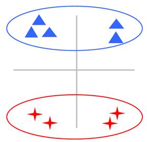
In many clustering problems, the input raw data sets often have a huge number of possible explanatory variables. However, not all features will help discover the cluster structure. Figure 1 gives a simple example to illustrate this scenario.
(a)
 .
.
(b)
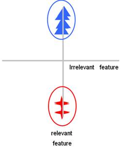
Figure 1: The effect of irrelevant feature in the clustering problem. The triangles and the stars are from two different groups in the 2-dimensional space. In (a), the two groups cannot be distinguished from the horizontal dimension. Besides, the points from the same group look a little far away. In contrast, in (b), after discarding the horizontal feature, the cluster structure becomes much more obvious, thus the clustering will be much easier and more accurate.
With the increase of the number of irrelevant features, the distance between the two points may be less reliable, the points which are near to each other in nature may artificially become far apart. Therefore, it is necessary to perform feature selection for the clustering algorithm.
In this project, a new feature selection method is proposed, through which not only the most relevant features are identified, but the redundant features are also eliminated so that the smallest relevant feature subset can be found. We integrate this method with our recently proposed Gaussian mixture (GM) clustering approach, namely rival penalized expectation-maximization (RPEM) algorithm [Cheung 2005], which is able to determine the number of components (i.e., the model order selection) in a Gaussian mixture automatically. Subsequently, the data clustering, model selection, and the feature selection are all performed in a single learning process.
2. Algorithm Description
2.1 Overview of GM Clustering and RPEM Algorithm
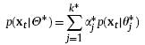
Suppose that N i.i.d. observations, denoted as XN={x1, x2, . . . , xN}, are generated from a mixture of k∗ Gaussian components, i.e.,
with
where each observation xt (1≤t≤N) is a column vector of d dimensional features: x1,t, . . . , xd,t. Furthermore, ![]() is the jth Gaussian component with the
parameter
is the jth Gaussian component with the
parameter ![]() ,
where
,
where ![]() and
and
![]() are
the true mean vector (also called center vector interchangeably) and covariance matrix of the jth component, respectively.
are
the true mean vector (also called center vector interchangeably) and covariance matrix of the jth component, respectively. ![]() is the true
mixing coefficient of the jth
component in the mixture. The main task of GM clustering analysis is to find an
estimate of
is the true
mixing coefficient of the jth
component in the mixture. The main task of GM clustering analysis is to find an
estimate of ![]() , denoted as
, denoted as ![]() , from N observations, where k is an estimate of the
true model order k∗. A general approach is to search in the
parameter space to find a
, from N observations, where k is an estimate of the
true model order k∗. A general approach is to search in the
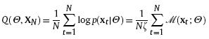
parameter space to find a ![]() that reaches a maximum of the fitness in
terms of maximum likelihood (ML) defined below:
that reaches a maximum of the fitness in
terms of maximum likelihood (ML) defined below:
![]()
The commonly used searching strategy is the EM algorithm. However, there is no penalty for the redundant mixture components in the above likelihood, which means that the model order k cannot be automatically determined and has to be assigned in advance. Although some model selection criteria have been proposed in the literature, they may require users to compare the candidate models for a range of orders to determine the optimal one, whose computation is laborious.
Recently, the RPEM algorithm [Cheung 2005] has been proposed to determine the model order automatically together with the estimation of the model parameters. This algorithm introduces the weights (whose values may be negative unlike the common non-negative weights) into the conventional likelihood; thus the weighted likelihood is written below:
with
![]()
where
![]()
is the posterior probability that xt belongs to the jth component in the
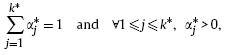
mixture, and k is greater than or equal to k∗. ![]() 's are designable weight
functions, satisfying the constraints below:
's are designable weight
functions, satisfying the constraints below:
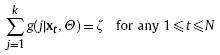
and
![]()
where z is a positive constant. In RPEM, they are constructed by the following equation (by simply setting z = 1):
![]()
with
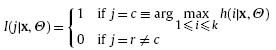
and et is a small positive quantity. This construction of weight functions reflects the pruning scheme: when a sample xt comes from a component that indeed exists in the mixture, the value of h(j|xt, Q) is likely to be the greatest, thus this component will be the winner, i.e., j = c with I(c|xt, Q) = 1. Accordingly, a positive weight g(c|xt, Q) will strengthen it in the temporary model. In contrast, all other components fail in the competition and are treated as the “pseudo-components”. As a result, the negative weights are assigned to them as penalties. Over the learning process of Q, only the genuine clusters will survive finally, whereas the “pseudo-clusters” will be gradually faded out from the mixture. The RPEM gives an estimation of Q* via maximizing weighted likelihood (MWL), i.e.,
![]()
2.2 Unsupervised feature selection
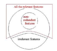
Figure 2 The configuration of all features.
The general configuration is described in Figure 2. Among all the features, some are irrelevant to the clustering. Furthermore, some relevant features may be redundant for the clustering task and can be further eliminated. Hence, we select the most possible relevant features at first, and then select the non-redundant features for the clustering.
2.2.1 Selecting the Relevant Features
We propose the following quantitative index to measure the relevance of each feature:
where ![]() is the variance of the jth cluster projected on the lth dimension:
is the variance of the jth cluster projected on the lth dimension:
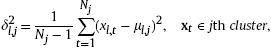
![]() is the number of data in the jth cluster, ml,j is the mean of the lth feature xl,t's in the jth cluster, and
is the number of data in the jth cluster, ml,j is the mean of the lth feature xl,t's in the jth cluster, and ![]() . Furthermore,
. Furthermore,![]() is the global variance of the
whole data on the lth dimension:
is the global variance of the
whole data on the lth dimension:
![]()
The ![]() measures the dissimilarity between
the variance in the jth cluster and the global
variance on the lth feature, which equivalently
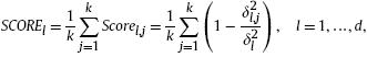
indicates the relevance of the lth feature for the jth cluster. Thus, SCOREl represents the average relevance
of the lth feature to the clustering
structure. When the value of SCOREl is close to the maximum value
(i.e., 1), it represents the case that all the local variances of the k clusters on this dimension are
considerably small in comparison to the global variance of this dimension,
which is tantamount to indicating these clusters far away from each other on
this dimension. Hence, this feature is very useful to detect the grouping
structure. Otherwise, the value of SCOREl will be close to the minimum
value, i.e., 0. To prevent the score from being degenerated in a situation that
measures the dissimilarity between
the variance in the jth cluster and the global
variance on the lth feature, which equivalently
indicates the relevance of the lth feature for the jth cluster. Thus, SCOREl represents the average relevance
of the lth feature to the clustering
structure. When the value of SCOREl is close to the maximum value
(i.e., 1), it represents the case that all the local variances of the k clusters on this dimension are
considerably small in comparison to the global variance of this dimension,
which is tantamount to indicating these clusters far away from each other on
this dimension. Hence, this feature is very useful to detect the grouping
structure. Otherwise, the value of SCOREl will be close to the minimum
value, i.e., 0. To prevent the score from being degenerated in a situation that
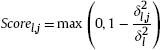
![]() is
greater than
is
greater than ![]() in
Eq. (6), which may be caused by numerical computation in computer, we clip the Scorel,j at 0. That is, we update Scorel,,j by
in
Eq. (6), which may be caused by numerical computation in computer, we clip the Scorel,j at 0. That is, we update Scorel,,j by
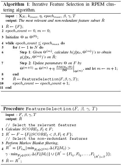
According to the score of each feature, we can obtain the selected relevant feature subset R in the following way:
![]()
where F is the full feature set and is a user-defined threshold value. By a rule of thumb, we set b ∈ [0, 0.5]. In the next subsection, we will further select the non-redundant features from R .
2.2.2 Selecting the Non-redundant Features
Based on the information theory, we know that a feature is redundant if it carries no additional partition information provided that the remaining features are presented. Hence, we are able to ignore it without compromising the model performance. Such an idea can be realized by a feature's Markov Blanket, which is originally proposed in the domain of supervised learning.
2.3 Iterative Feature Selections in the RPEM Algorithm
Since the optimal number of clusters and the optimal feature subset are inter-related, we integrate the feature selection schemes into the RPEM algorithm so that the feature selection and the clustering process are performed iteratively in a single learning process. Specifically, given a feature subset, we run the RPEM algorithm by scanning all observations once (i.e., one epoch) and obtain a near optimal partition. Then, the proposed feature selection scheme outputs a refined feature subset in terms of the relevance and non-redundance under the current data partition. Subsequently, a more accurate partition will be performed using the selected feature subset in the next epoch. Algorithm 1 presents the details of the proposed algorithm.
3. Experimental Results
3.1 Synthetic Data
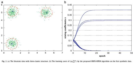
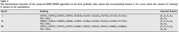
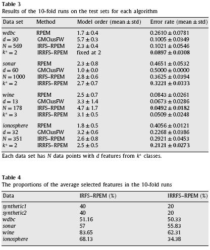
Firstly, we investigated the capability of the proposed algorithm to select the relevant and non-redundant features while determining the correct number of clusters simultaneously. As shown in Fig. 2(a), 1000 data points were generated by a bivariate GM. In Fig. 2(a), we are unable to discriminate the three clusters by a single dimension alone. Actually, both features are relevant to the clustering. We duplicated the two dimensions and formed a four-dimensional data. Each data were further appended with six independent variables that were sampled from a standard normal distribution and finally yielding a 10-dimensional data set to be analyzed. Apparently, either {F1, F2} or {F3, F4} can determine the three clusters, i.e., one of the two pairs of features are redundant. The last six dimensions are unimodal, thus being irrelevant to the clustering. Table 1 summarizes the results in the evolution.
3.2 Real-world Data
We further investigated the performance of the proposed algorithm on four benchmark real-world data sets from UCI repository. We normalized the mean and variance of each data set to 0 and 1, respectively. For comparison, we also performed the RPEM algorithm, GMClusFW algorithm [Law et al. 2004], and a variant of the proposed algorithm (denoted as IRFS–RPEM) that carried out the relevancy analysis only in the feature selection phase without considering the feature redundancy. The same weight functions were chosen for RPEM, IRFS–RPEM and IRRFS–RPEM.We evaluated the clustering accuracy using the index of error rate. The mean and the standard deviation of the error rate, along with those of the estimated number of clusters in 10-fold runs on the four real-world data sets are summarized in Table 3.
4. References
1. Y.M Cheung, “Maximum Weighted Likelihood via Rival Penalized EM for Density Mixture Clustering with Automatic Model Selection”, IEEE Transactions on Knowledge and Data Engineering, 17(6), pp. 750-761, 2005.
2. M. Law, M. Figueiredo, A. Jain, “Simultaneous Feature Selection and Clustering Using Mixture Models”, IEEE Transactions on Pattern Analysis and Machine Intelligence, 26(9), pp. 1154-1166, 2004.
5. Selected Publication
H. Zeng and Y.M. Cheung, “A New Feature Selection Method for Gaussian Mixture Clustering”, Pattern Recognition, 42 (2009) 243-250.